
RESEARCH ARTICLE
Joint Probability Distribution Functions for the Filtered Velocity Gradient Invariants in Homogeneous Isotropic Turbulence
Waleed Abdel Kareem1, *, Mahmoud Abdel Aty2, Zafer M. Asker1
Article Information

Identifiers and Pagination:
Year: 2018Volume: 12
Issue: Suppl-1, M4
First Page: 54
Last Page: 66
Publisher Id: TOMEJ-12-54
DOI: 10.2174/1874155X01812010054
Article History:
Received Date: 25/05/2017Revision Received Date: 10/07/2017
Acceptance Date: 17/07/2017
Electronic publication date: 15/02/2018
Collection year: 2018
open-access license: This is an open access article distributed under the terms of the Creative Commons Attribution 4.0 International Public License (CC-BY 4.0), a copy of which is available at: (https://creativecommons.org/licenses/by/4.0/legalcode). This license permits unrestricted use, distribution, and reproduction in any medium, provided the original author and source are credited.
Abstract
Background:
Turbulent flow is characterized by vortices with different scales. Extraction of various scales and filtering the turbulent field into coherent and incoherent parts are important processes that improve our understanding of turbulent characteristics.
Objective:
Joint probability distribution functions (JPDFs) for the filtered velocity gradient invariants are extensively studied for different scales as well as for the coherent and incoherent parts of each scale.
Methods:
The Fourier decomposition and the anisotropic diffusion model are used in the investigation. The extraction process is performed by employing the Fourier decomposition at different cutoff wavenumbers for the velocity field and three distinct scales (large, medium and fine scale) are identified. The velocity gradient invariants such as the second invariant Q and the third invariant R for the different scales are extracted. Then other important invariants such as the rate of rotation tensor QW and the rate of deformation QS are also identified for each scale. The anisotropic diffusion model is used to extract the coherent and incoherent parts of each invariant at each scale. Then the JPDFs of the coherent and incoherent invariants are compared. The scale decomposition and the filtering process are applied for turbulent flow fields that are simulated using the lattice Boltzmann method with resolution of 1283.
Results:
Results show that the (R-Q) space has a universal topological pear-like shape for the different scales as well as their coherent field. However, the (R-Q)-space for the incoherent fields are found different and no general shape can be observed. The (Qw-QS)-space results show self-similar shapes for coherent fields and for the incoherent fields no specific shape can be observed since the noise distributed as separated points everywhere.
Conclusion:
Two different methods for extraction and filtering of forced isotropic turbulence and the JPDFs of the velocity gradient invariants are studied. Some universal characteristics for the coherent parts were found. However, for the incoherent parts, no universal JPDFs were found.
1. INTRODUCTION
Most fluid flow problems are turbulent and the presence of coherent structure inside a flow field encourages more researchers to investigate statistical turbulent flow analysis methods such as the extraction and filtering methods. Filtering turbulent field to coherent and incoherent parts are commonly based on the wavelet and Fourier decompositions. One of the filtering methods is the coherent vorticity extraction (CVE) method. CVE which is based on a wavelet analysis was introduced by Farge et al. [1, 2]. Wavelet is one of the attractive mathematical features, and it was used in the 1990s by M. Farge et al. [3, 4] to identify coherent vortices in 2D isotropic turbulence. Wavelet methods in computational fluid dynamics have been reviewed by Schneider and Vasilyev [5]. M. Farge et al. [3] used the continuous wavelet transform to explore the coherent structure of turbulent flows. Abdel Kareem et al. [6] used two different methods, the Fourier band-pass cutoff process and the wavelet decomposition to extract large, intermediate and fine scales. The partial differential equations (PDEs) are used widely in various branches of sciences such as R. Malladi, J. Sethian [7], where they are used as a class of PDE-based algorithms to enhance images, to remove noise and to recover objects in the processed image. The extracted coherent and incoherent parts using the fourth order (PDEs) from a turbulent flow field were studied by Abdel Kareem [8]. Also, Abdel Kareem et al. [9] identified the coherent vortices of various scales from a turbulent flow field obtained by a direct numerical simulation (DNS using sharp cut-off filters before the vortex-identifying method. Perona and Malik introduced nonlinear noise removal algorithm [10], which at first was used in image processing and restoration. Because of the need for better performance, edge-preserving and efficient noise-removing than Perona and Malik algorithm, Mahmoodi developed a new partial differential equation model based on Perona and Malik algorithm [11]. Abdel Kareem et al. [12] generalized the model [11] to a three dimension model to extract the coherent and the noise parts from 3D turbulent flow fields.
The extraction process depends on identifying different scales in the flow field by using an appropriate decomposition such as the Fourier decomposition which divides the velocity field to large, intermediate and fine scales. In Fourier decomposition the velocity field converted into Fourier space, and at different cutoff wave numbers, the different Fourier modes for different scales are obtained. Finally the extracted velocity data is returned to the physical space. M. Farge et al. [13] used the coherent vortex extraction (CVE) and the proper orthogonal decomposition to compare the wavelet and the Fourier decomposition in identifying coherent and incoherent parts. Abdel Kareem et al. [14] extracted different flow field scales by Fourier decomposition and tracked it at different scales.
Turbulent flow is one of the important subjects in fluid studies, so many of researchers were dedicated to explore the formation and structure of turbulence in fluids. In the previous efforts, the velocity gradient tensor was used to investigate many universal characteristics, so Chong, Perry and Cantwell introduced the invariants R and Q [15] to study the topological features of turbulence. Soria and Cantwell [16], Cantwell [17] and Ooi et al. [18] used the topological approach to study the structures of the velocity gradient tensor (Δu), the rate of strain tensor QS and rotation tensor QW by investigating the tensors invariants. The topological methodology was applied by Chen et al. [19] to study the turbulent mixing layer flows. This topological method is used in this study against different scales and for the coherent and incoherent parts. Also, the joint PDFs are applied to the extracted and filtered data divided into different scales with their coherent and incoherent parts.
The paper is organized as follows. In section 2, the generation of the turbulent flow data by the lattice Boltzmann method and the invariants of the velocity gradient tensor are introduced. In section 3, the Fourier decomposition to extract different flow field scales is discussed. In section 4, the anisotropic filtering method for turbulent flow fields is formulated. Section 5 is devoted to the results and discussions of the obtained features. The last section, Sec. 6, summarizes the conclusions of the study.
2. TURBULENT FLOW FIELDS
2.1. The Lattice Boltzmann Simulation
The lattice Boltzmann method (LBM) and the spectral method that used to solve the Navier-Stokes equations are important tools in the simulations of fluid dynamics problems. Many researchers used the lattice Boltzmann method in turbulence studies (Yu et al. [20], Devaraj et al. [21] and Abdel Kareem et al. [22]).
More details about the derivation of the lattice Boltzmann equation from the Navier-Stokes equations can be found in the previous works, which were introduced by Chen et al. [23]. The LBM depends on considering the fluid as a group of particles instead of considering it as a continuous matter. These particles move in a lattice only from one node is the discrete velocity set in the of 1283, Abdel Kareem et al. [24], used the LBM for forced turbulence flow simulations. This turbulent flow data are used in the investigation. The lattice Boltzmann equation and definitions of distribution functions, densities, velocities and equilibrium distribution function were presented in many previous publications such as by Succi [25], where he discussed the lattice Boltzmann equation theory, its fluid dynamics applications, and its major applications. The Lattice Boltzmann equation can be written as:
 |
(1) |
where the distribution function in the equilibrium state can be given as:
 |
(2) |
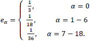
and eα is the discrete velocity set in the D3Q19 model defined as:
 |
(3) |
Respective weighting coefficients ωα in this case are defined by:
 |
(4) |
2.2. Invariants of the Velocity Gradient Tensor
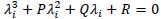
The velocity gradient tensor A or Aij = ∂ui/∂xj, has the following characteristic equation:
 |
(5) |
where λi, P, Q and R are the first, second and third invariants of A, respectively. The definition of these invariants can be written as follows
 |
(6) |
 |
(7) |
 |
(8) |
In incompressible flow case  .U= ∂ui/∂xi = Aii = 0, the corresponding tensor invariants can be given as
 |
(9) |
 |
(10) |
and
 |
(11) |
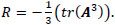
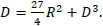
Also, the discriminant for Aij in incompressible flow is defined as:
 |
(12) |
Now the velocity gradient tensor can be split into a symmetric component and a skewsymmetric component:
 |
(13) |
where Sij is the symmetric rate of strain tensor and Wij is the antisymmetric rate of rotation tensor which is given by:
 |
(14) |
 |
(15) |
Using the invariants Sij and Wij, the tensors Q and R can be defined as
 |
(16) |
 |
(17) |
Q and R can be divided into the strain components Qs, Rs and the rotation components QW and RW as follows:
 |
(18) |
where
 |
(19) |
 |
(20) |
where these different invariants can be described as follows(see [26-31])
- QS is the rate of deformation or stretching tensor and QW is the rate of rotation or vorticity tensor.
- QW is always positive and QS is always negative.
- The (QW –QS) map and topological classifications are shown in Fig. (1), QW = -QS represents the 45o line [29].
- The discriminant D value (Eqn. 10) determines the eigenvalues of A: D > 0 gives one real and two complex-conjugate eigenvalues; D < 0 gives three real and distinct eigenvalues.
- The (R-Q) map and topological classifications of local flow fields are shown in Fig. (2) [30] where D = 0 or R=(±2 (√3)/9)(-Q3/2) gives the tent like curve.
- The region R < 0; Q > 0 is associated with vortex stretching.
- The region R > 0; Q > 0 is associated with vortex compression.
- The region R < 0; Q < 0 is associated with tube structures.
- The region R > 0; Q < 0 is associated with sheetlike structures.
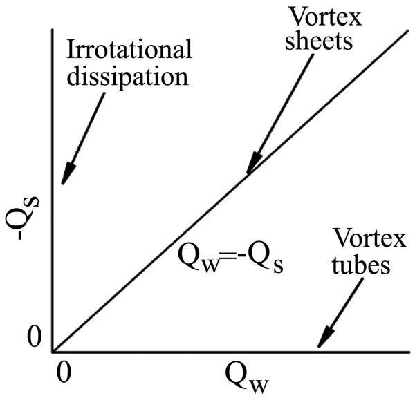 |
Fig. (1). The invariant physical map of (QW -QS) for incompressible flows [29]. |
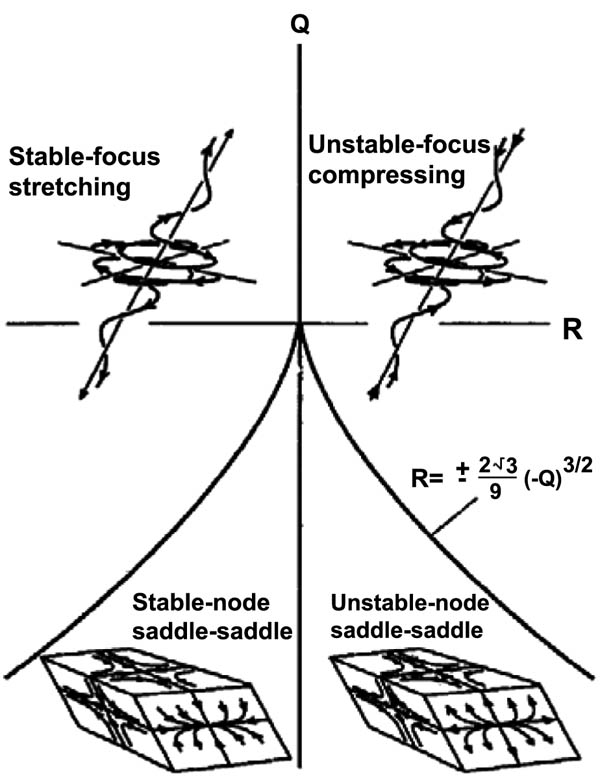 |
Fig. (2). The local (R -Q) topologies for incompressible flows [30]. |
3. FOURIER DECOMPOSITION
The fast Fourier transform (FFT) over all physical space coordinates is defined by
 |
(21) |
and the inverse Fourier transform can be written as
 |
(22) |
the last summation is over all wavenumbers in Fourier space. Using the following different cutoff frequencies the velocity field can be decomposed into different scales in Fourier space using band pass cutoff as follows
| scales | Large scale | Medium scale | Find scale |
|---|---|---|---|
| symbols | UL | UM | UF |
| cutoff | 0< k < k1 | k1 < k < k2 | k2 < k < k3 |
Depending on the results of a previous study [6], the cutoff wavenumbers are chosen as k1 = 4, k2 = 12, k3 = 60 for the resolution of 1283 case. Those cutoffs are used also in this study to identify the large, the intermediate and the fine scales.
4. THE ANISOTROPIC DIFFUSION MODEL
Sasan Mahmoodi [11] proposed an algorithm which demonstrates better performance for band pass noisy signals containing discontinuities depending on Perona and Malik algorithm [10]. This anisotropic diffusion model is considered to extract coherent and incoherent parts from a 3D isotropic turbulent flow field. In this study, the 3D model is applied to decompose the flow field as follows
- Large scale velocity UL = ULc + ULinc,
- Medium scale velocity UM = UMc + UMinc,
- Fine scale velocity UF = UFc + UFinc .
The model can be written as
 |
(23) |
the total real term can be written as
 |
(24) |
The total imaginary part is defined as
 |
(25) |
the real functions  are defined as
 |
(26) |
 |
(27) |
The imaginary functions  are defined as
 |
(28) |
 |
(29) |
The functions  are defined as
 |
(30) |
Where the functions  are defined as
 |
(31) |
 |
(32) |
Finally the functions  can be defined as
 |
(33) |
Where the function U(x, y, z, t) is defined as
 |
(34) |
Here  is the original signal. The detailed derivation of the 3D model and the application of the Fourier decomposition to extract the different scales and the filtered fileds with their visualization can be found in [32].
5. RESULTS AND DISCUSSIONS
The velocity field  is extracted to the components L, M and F. after using the Fourier decomposition as explain in section 3, then the extracted velocity L is divided into coherent part LC and incoherent part Linc. The same is done for the extracted velocities M and F, respectively.
- The extraction of different invariants can be summarized as
- For L we calculate QL, RL, QWL, and QSL.
- For M we calculate QM, RM, QWM, and QSM.
- For F we calculate QF, RF, QWF, and QSF .
- For
- The filtered invariants are identified as follows
- For LC we calculate QLC, RLC, QWLC and QSLC
- For MC we calculate QMC, RMC, QWMC and QSMC
- For FC we calculate QFC, RFC, QWFC and QSFC
- For Linc we calculate QLinc, RLinc, QWLinc and QSLinc
- For Minc we calculate QMinc, RMinc, QWMinc and QSMinc
- For Finc we calculate QFinc, RFinc, QWFinc and QSFinc
- For
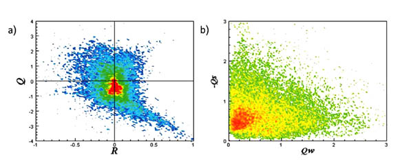 |
Fig. (3). JPDFs: (large scale) (a) The (RL –QL); (b) The (QWL –QSL). |
5.1. JPDFs RESULTS
The results for the joint PDFs in the extracted data, show that in L (Fig. 3a), M (Fig. 4a) and F (Fig. 5a), pear-like shape appear clearly in the (R-Q) plane. These results are similar to previous studies [30]. Where there is a kind of universality in the (R-Q) invariant space is found. The strong anti-correlation between R and Q can be observed in the region (R > 0, Q < 0) with sheet structure, however in the region (R < 0, Q > 0) vortex stretching can be shown. In the (R-Q) plane, for the left side, the points are classified as stable, and in the right side of the plane, the points are classified as unstable. Actually this physical interpretation concluded from the (R-Q) map helps us to explain the local flow topology, vortex stretching or vortex compression and contraction or expansion. In the (QW-QS) case (Figs. 3b, 4b and 5b), a self-similar shape appears regardless of the filtered scale, which also in good agreement with previous studies, where the horizontal line QW implies the points with the vortex tube structure, while the vertical line -QS represents the points with irrotational strain fields. The 45o line with QW = -QS represents the vortex sheet structures, or points with a high dissipation that accompanied with a high enstrophy density.
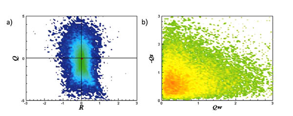 |
Fig. (4). JPDFs: (medium scale) (a) The (RM –QM); (b) The (QWM –QSM). |
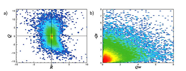 |
Fig. (5). JPDFs: (fine scale) (a) The (RF –QF); (b) The (QWF –QSF). |
The joint PDFs for filtering results, in the coherent part LC, MC and FC, because the vortices presence, it is clear that the results are generally similar to the turbulent scales (L, M and F), where pear-like shape is observed in (R-Q) plane (Figs. 6a, 7a and 8a). The (QW-QS) plane results (Figs. 6b, 7b and 8b), a self-similar shape appeared. But in the incoherent part for different scales, Linc, Minc and Finc, because absence of the vortices, there are just noise points scattered everywhere; there is no specific shape can be extracted in the (R-Q) or the (QW-QS) planes. We can observe for the large and the medium incoherent (R-Q) plane in focal region and the R = 0 axis, a bulk of data (Figs. 9a and 10a), and in fine incoherent (R-Q) (Fig. 11a) more noise points scattered in a wide area without specific shape, These points increase in the negative area. For (QW-QS) plane in large and medium incoherent field (Figs. 9b and 10b) noise points propagate in an area like that extracted in Figs. (3b and 4b) for the large and medium scales or their coherent cases (Figs. 6b and 7b) where their existence is concentrated in the center and at small values and decreased with positive values, as shown in Fig. (11b) where noise points are concentrated in a right-angled triangle shape and decreased in remaining area.
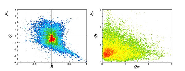 |
Fig. (6). JPDFs: (large coherent part) (a) The (RLc –QLc); (b) The (QWLc –QSLc). |
 |
Fig. (7). JPDFs: (medium coherent part) (a) The (RMc –QMc); (b) The (QWMc –QSMc). |
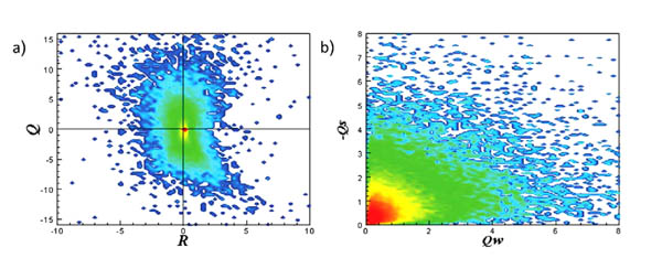 |
Fig. (8). JPDFs: (fine coherent part) (a) The (RFc –QFc); (b) The (QWFc –QSFc). |
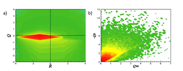 |
Fig. (9). JPDFs: (large incoherent part) (a) The (RLinc –QLinc); (b) The (QWLinc –QSLinc). |
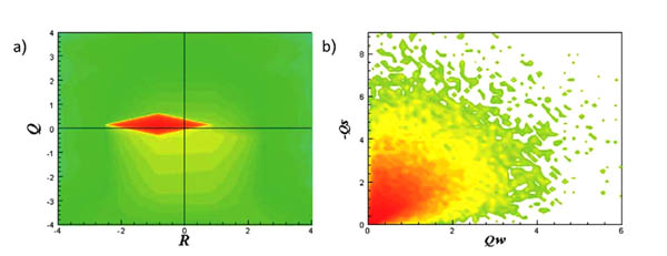 |
Fig. (10). JPDFs: (medium incoherent part) (a) The (RMinc –QMinc); (b) The (QWMinc –QSMinc). |
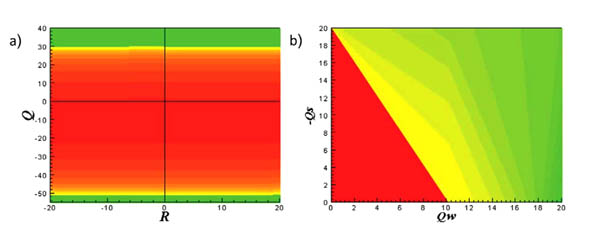 |
Fig. (11). JPDFs: (fine incoherent part) (a) The (RFinc –QFinc); (b) The (QWFinc –QSFinc). |
CONCLUSION
The Fourier decomposition was used to extract different scales and the anisotropic diffusion model was used to identify the coherent and noise parts of the different scales. Separating the coherent vortices from noisy parts are important and useful for studying and tracking individual vortices, dividing the flow field into different scales helps in studying huge data and understanding energy transformation. By studying the JPDFs for different scales and their corresponding coherent and incoherent parts a confirmation of the pear-like shape in the (R-Q) plane for the different scales and their coherent part was presented. However the incoherent (R-Q) planes gave undefined shape, these results are in good agreement with previous turbulent studies and indicate that the vortices are the main components of turbulent motion.
There are some issue that not addressed in this study and can be considered at future work such as study the JPDFs for boundary layer structures and investigation of the coherent and incoherent JPDFs in high resolution turbulent data that obtained by simulations or that simulated by solutions of the Navier-Stokes solution.
CONSENT FOR PUBLICATION
Not applicable.
CONFLICT OF INTEREST
The authors declare no conflict of interest, financial or otherwise.
ACKNOWLEDGEMENTS
Declared none.