
RESEARCH ARTICLE
Growth of Spiral Vortices in a Globally Unstable Region on a Rotating Disk
Lee Keunseob*, Nishio Yu, Izawa Seiichiro, Fukunishi Yu
Article Information

Identifiers and Pagination:
Year: 2018Volume: 12
Issue: Suppl-1, M2
First Page: 22
Last Page: 36
Publisher Id: TOMEJ-12-22
DOI: 10.2174/1874155X01812010022
Article History:
Received Date: 23/05/2017Revision Received Date: 14/06/2017
Acceptance Date: 20/06/2017
Electronic publication date: 15/02/2018
Collection year: 2018
open-access license: This is an open access article distributed under the terms of the Creative Commons Attribution 4.0 International Public License (CC-BY 4.0), a copy of which is available at: (https://creativecommons.org/licenses/by/4.0/legalcode). This license permits unrestricted use, distribution, and reproduction in any medium, provided the original author and source are credited.
Abstract
Background:
Instabilities on a rotating disk flow can be classified into two distinct groups, convective instability and global instability. Contrary to the convective instability, many characteristics of the global instability are left unknown despite of a lot of researches.
Objective:
The study investigates the characteristics of the globally unstable mode.
Method:
Numerical simulation is carried out by a finite difference method. The simulation code solves the full Navier-Stokes perturbation equations and the continuity equation.
Results:
Four cases with azimuthal domain sizes of 2π/10, 2π/70, 2π/80 and 2π/90 are compared. In all cases, a short-duration wall-normal random suction and blowing is introduced from the wall at the beginning of the computation. In the computation for the wider size 2π/10 domain, wavenumber components of 70, 80 and 90 are all found to co-exist in the flow field, with the wavenumber 80 component being much stronger than the other two components. The strength of the wavenumber 80 component is equivalent to the narrower domain case. For the other two wavenumber components of 70 and 90, the strengths in the wider domain case are much lower compared to the corresponding narrower domain cases. When the same wavenumber components are compared between the wider and narrower domain computations, no difference can be found, indicating that each wavenumber component grows by the global instability.
Conclusion:
The results imply that the amplitude saturation levels of wavenumber components 70 and 90 are suppressed by the wavenumber 80 component through the nonlinear effect.
1. INTRODUCTION
The 3-D boundary layer transition over a rotating disk is studied due to its resemblance to a swept wing. The boundary layer over a rotating disk becomes three-dimensional because of the centrifugal force. Thus the transition process on a rotating disk is basically the same as that on a swept wing flow. Instabilities on a rotating disk flow can be classified into three distinct groups. Convective instability in which the amplitude of disturbances develop as they move downstream is the most common in the experiments because unavoidable minute roughness on a real disk introduces a continuous disturbance into the boundary layer. Moreover, once the flow is disturbed in these unstable regions, the absolute instability and global instability will make the flow continually unstable even after the disturbance vanishes.
To investigate convective instability, Smith [1] in an experiment used random disturbances to excite the boundary layer and detected sinusoidal waves in the transition region for the first time. Gregory et al. [2] clearly showed 28  32 equi-angular spiral vortices at a Reynolds number of around 430. Fedorov et al. [3] observed that the different types of vortices were overlapped on the disk surface. Kobayashi et al. [4] and Kohama [5] observed ring-like co-rotating vortices around a spiral vortex were excited and concluded that the ring-like co-rotating vortices caused the rapid transition by smoke flow visualization. An experimental study by Wilkinson & Malik [6] using a hot-wire showed that discrete roughness disturbance on the disk excites the spiral vortices and that the secondary instability was also observed before turbulent breakdown. Corke & Knasiak [7] conduced an experiment in which the artificial roughness on the disk was organized to control the characteristics of the stationary modes and confirmed that the travelling mode and stationary mode were coupled in the nonlinear stage.
Theoretical studies on the transition process of the rotating disk have also been conducted. Kobayashi et al. [4] and Malik et al. [8] reported that the critical Reynolds numbers for the stationary cross-flow instability were 261 and 287, respectively, based on their experimental and theoretical studies. They insisted that the gap between theoretical results and experimental results for the critical Reynolds number could be decreased when the effect of Coriolis force and the streamline curvature were included in the linear stability theory. Malik [9] used a theoretical approach and showed that the critical Reynolds numbers of the stationary mode for the inviscid type was 285.36 and that of the viscous type was 440.88. Balakumar & Malik [10] also showed that the critical Reynolds numbers for the traveling mode were 283.6 for the inviscid type and 64.46 for the viscous type. Hussain et al. [11] investigated the stationary and the traveling modes of the inviscid type and the viscous type for the convective instability by the theoretical method. They found that although the cross-flow instability was the most amplified, the streamline-curvature instability was also important in an axial flow. It should be noted that the experimental results are in good agreement with the theoretical results for the convective stationary instability of the stationary mode, even though other instabilities are also disturbing the rotating disk flow.
Following the researches on convective instability, a theoretical study by Lingwood [12, 13] suggested that the absolute instability contributes to the rapid transition downstream of the Reynolds number of 507. In the investigations, the parallel-flow assumption was applied. However, it was found that the results would be different if the target of the investigation was the global instability instead of the absolute instability. Itoh [14, 15] used the theoretical method and employed the vicinity of the singularity point for the zero complex group velocity. He showed that the flow field under the slightly non-parallel-flow condition was absolutely stable, and therefore concluded that applying the parallel-flow assumption is not proper. In addition, the numerical simulations performed by Davies & Carpenter [16] showed that an artificial disturbance grew upstream starting from its introduced location, but consequently the convectively unstable mode became dominant. Moreover, Othman & Corke [17] used an air pulse to introduce the disturbance and found that the wave packet simply grew in a linear fashion without any abrupt change in the amplitude near the critical Reynolds number for the absolute instability, which was 507. Therefore, although there are cases where the global instability causes velocity fluctuation to grow, a clear evidence which shows the direct contribution of the absolute instability does not exist. Prior to the study by Appelquist et al. [18], studies on the global instability focused on Re = 507, which was the critical Reynolds number for the absolute instability. However, Appelquist et al. [18] suggested that the critical Reynolds number for the global instability is Re = 583, based on direct numerical simulation on full Navier-Stokes equations.
In our present study we conducted a numerical simulation on full Navier-Stokes equations to investigate the characteristics of the globally unstable mode. Numerical simulation can deal with a clean disk surface, and thus it was the best tool for use in this study, because in experiments, roughness on a disk surface introduces a continuous disturbance that is grown by the convective instability. The remainder of this paper is organized as follows. The numerical method and conditions are shown in section 2. Section 3 presents the results of two cases in which the computational domains for the azimuthal direction are different. Our conclusions are given in section 4.
2. NUMERICAL FORMULATION AND NUMERICAL PROCEDURES
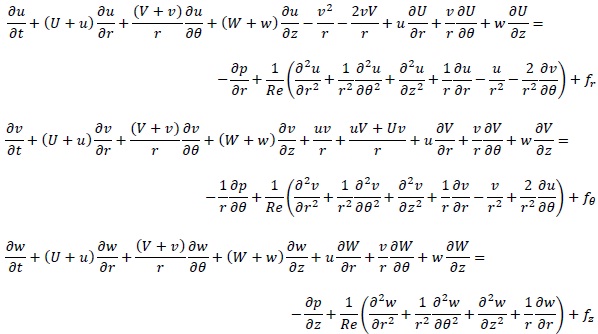
Numerical simulation is carried out by a finite difference method. The simulation code is self-developed, and solves the full Navier-Stokes perturbation equations,
 |
(1) |
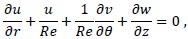
and the continuity equation,
 |
(2) |
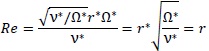
where u = (u, v, w) are the radial, azimuthal and wall-normal components of the perturbation velocities, and U = (U, V, W) are those of the corresponding base-flow velocities in cylindrical polar coordinates. The base flow is given by the von Kármán similarity solutions [19], which are obtained by solving a set of ordinary differential equations using the forth-order Runge-Kutta method. t is time, p is a fluctuating component of pressure, and a forcing term f (= (fr, fθ, fz)) is used in the sponge regions. All the variables in the above equations are nondimensionalized by the length  , the rotational velocity r*Ω*, the time scale r* / (r*Ω*) and the pressure (r*Ω*)2ρ, where ν is the kinematic viscosity, ρ is the density, Ω* is the angular velocity, and the superscript * denotes dimensional values. Thus, the Reynolds number in the simulations is defined as
 |
(3) |
which reveals that the nondimensional radial position r on the disk is identical to this Reynolds number Re. Hereafter, the number of disk rotations, given by T = t*Ω* /2π, is used to scale time.
The full Navier-Stokes perturbation equations and the continuity equations are solved by the MAC method (marker and cell method), which solves a Poisson equation to obtain the pressure and then computes the velocities using the Navier-Stokes equations. The second-order Crank-Nicolson semi-implicit scheme is applied for time advancement. The third-order upwind scheme (K-K scheme [20]) is used in the convection terms, and the fourth-order central difference scheme is used for the other terms. For the Poisson equation, a 27-color SOR method is used, since our program is coded in CUDA to be used in a multi-GPU platform.
2.1. Computational Domain
Fig. (1) illustrates the computational domain, and Table 1 lists the computational parameters. The domain is a fan-shaped region instead of a full circular disk for the purpose of reducing the computational cost. The domain covers the region of 330 ≤ r ≤ 751, 0 ≤ θ ≤ 2π/β and 0.0 ≤ z ≤ 22.4. For the azimuthal direction, periodic boundary conditions are employed, and the azimuthal division number β is chosen as 10 at minimum. When β is equal to 10, the azimuthal angle of the domain is 2π/10, which can handle the azimuthal wavenumber of 10 and its multiples. Domains narrower in the azimuthal direction, 2π/70, 2π/80 and 2π/90 are also prepared for comparison to discuss the effect of periodic boundary conditions on the growth of velocity fluctuations. In the narrower domain cases, only each azimuthal wavenumber β = 70, 80 and 90 and its harmonics can be resolved, so that the interaction among the wavenumber components are restricted compared with the former case. The four cases with different azimuthal domain sizes will be compared throughout this research. For the wall-normal direction, the grids are distributed according to a geometric series of a common ratio of a and a starting wall-normal location of z0 . The wall-normal location is defined as
| β | (r,θ, z) | Nr × Nθ × Nz | (∆r,∆θ,z0 ,a) | |
 |
10 |
r [330,751] [330,751]θ [0,22.4] |
422 × 469 × 50 |
∆r = 1 ∆θ = |
 |
70 |
r [330,751] θ [0,22.4] |
422 × 73 × 50 |
∆r = 1 ∆θ = |
 |
80 |
r [330,751] θ [0,22.4] |
422 × 61 × 50 |
∆r = 1 ∆θ = |
 |
90 |
r [330,751] θ [0,22.4] |
422 × 61 × 50 |
∆r = 1 ∆θ = |


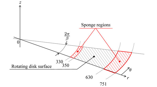 |
Fig. (1). Computational domain. |
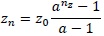 |
(4) |
where the n-th grid number is nz in the wall-normal direction. The values of z0 and a are given in Table 1. It should be noted that we have performed several computations by changing the size of domains in both the radial and the wall-normal directions, and confirmed that computational domains are large enough to elucidate the phenomena.
2.2. Initial Condition and Boundary Conditions
For the initial condition, the von Kármán similarity solution is adopted for the base velocity components, and for the perturbation velocities and pressure, these components are all set to zero. For the boundary conditions, the perturbation components at the upper boundary are set as u = 0, v = 0 and dw/dz = p, which is identical to those in Appelquist et al. (2016). The perturbation velocities are zero at the upstream and downstream boundaries in the radial direction. The periodic boundary condition is used in the azimuthal direction. The Neumann condition for the pressure is applied at all boundaries except for the upper boundary. In addition, sponge regions are introduced in order to prevent nonphysical reflections at the upstream and downstream boundaries. The sponge regions are located at both the upstream and downstream boundaries. The sponge function is given by
 |
(5) |
where the λ(Re) is defined as
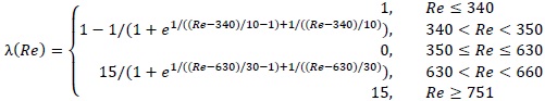 |
(6) |
Therefore, the actual computational region is from Re = 350 to Re = 630. In the sponge regions, the perturbation velocities are compulsorily diminished.
2.3. Artificial Disturbance
The characteristics of the nonlinear global instability of rotating disk flows were studied by focusing on the impulsive response against a random disturbance added from the disk surface for a very short time. The random disturbance is given in the form of a wall-normal suction and blowing, which is defined as
 |
(7) |
where wT(T), wr(r) and wa(θ) are the temporal, the radial and the azimuthal functions, respectively. The functions wT(T) and wr(r) are given by
 |
(8) |
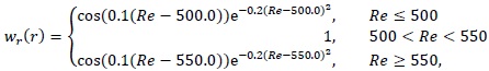 |
where 330 < r < 751 and 0.00 < T < 0.01. Fig. (2) shows the temporal amplitude and the radial amplitude for the artificial disturbance. At T = 0.00211, the temporal amplitude is maximum. The location where the artificial disturbance is introduced, Re ≈ 500 550, is lower than the critical Reynolds number for global instability Re = 583 [18]. The function wa(θ) has random values between -0.00001V and 0.00001V, where V is the rotating disk speed at the radial location. It should be noted that the azimuthal amplitude of each grid point is different, and is changed every time step.
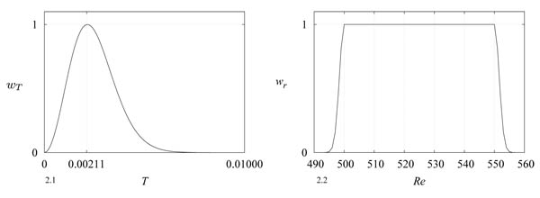 |
Fig. (2). The temporal amplitude of the artificial disturbance, wT(T). The radial amplitude of the artificial disturbance, wr(r). |
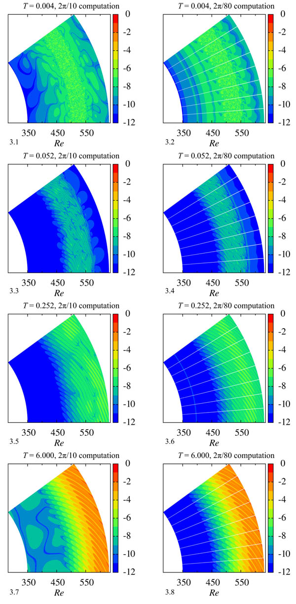 |
Fig. (3). Color maps of log |v| at z = 1.3. The wider computational domain case (2π/10) and narrower computational domain case (2π/80) are compared. |
3. RESULTS AND DISCUSSION
The present study focuses on the behavior of a wave packet generated by random suction and blowing at the disk surface whose location is stable to the global instability mode. Fig. (3) shows the time variation of the color map of log|v| at z = 1.3 when the wider domain of 2π/10 is used. The results of the computation using the narrower domain of 2π/80 are also shown for comparison. The sponge regions are placed inside and outside of the visualized region, Re = 330350 and 630721, which prevents contamination by undesirable reflections at the inflow and outflow boundaries. Immediately after a random disturbance is introduced into a boundary layer for a short time, a disturbed flow region with no characteristic pattern appears around the area of Re = 500550. This is regardless of the azimuthal size of the computational domain. However, after a short time, a finger-like pattern starts to form in this disordered region. At T = 0.252, stripe patterns can clearly be observed downstream of Re > 460. It should be noted that some irregularity is present in the wider domain computation. Here, two finger-like patterns of azimuthal velocity fluctuations correspond to one spiral vortex. At the later time of T = 6.0, 80 spiral vortices are present in the boundary layer in both the narrower domain (2π/80) case and the wider domain (2π/10) case. Lingwood (1995), on the basis of parallel flow assumption, theoretically predicted that the flow becomes absolutely unstable at Re > 507 and the critical azimuthal wavenumber is 68. Pier and Huerre (2001) pointed out that nonlinear global instability takes place as soon as local absolute instability arises at some point in the flow field, and thus, the nonlinear global mode with a sharp front, the so-called elephant mode, is governed by a local linear criterion. These results suggest that the azimuthal wavenumbers around 68 should be predominant as a primary wavenumber. In the wider domain (2π/10) computation, the components with azimuthal wavenumbers which are multiples of 10, including 60, 70, and 80, are all likely to appear. However, it was the wavenumber 80 component, not the wavenumber 70 component, which appeared as a dominant pattern in our computation. This discrepancy might be because the local stability theory cannot treat the competition of several wave packets that are localized in both the radial and azimuthal directions, as shown in Fig. (3.3).
Fig. (4) shows the spatial and temporal developments of velocity fluctuations log(vrms) at z = 1.3. The data are not filtered by the wavenumber. In all cases, the short-duration random disturbances were introduced at Re = 500550, which was within the globally stable region, only at the start of the computation (T =0.0 0.01). The patterns in the wider domain case (2π/10) and narrower domain cases (2π/70, 2π/80 and 2π/90) are similar. The weak velocity fluctuations first convect downstream, amplified by the convective instability. After T = 1.5, the contour lines are tilted in the upstream direction. This change implies that the velocity fluctuations began to be temporally amplified at the location by the global instability. It should be noted that at T = 6.0, the growths of the fluctuations are nearly saturated and the flow field becomes steady, in all cases.
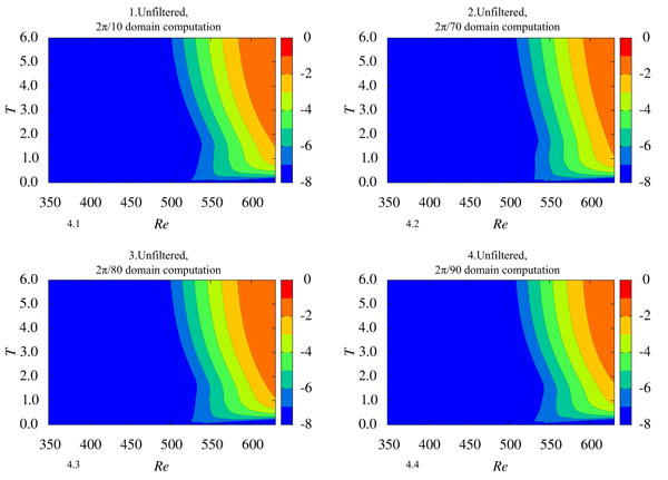 |
Fig. (4). Spatio-temporal development of log(vrms) at z = 1.3. (1) 2π/10 domain computation, (2) 2π/70 domain computation, (3) 2π/80 domain computation, (4) 2π/90 domain computation. |
Fig. (5) shows the power spectra of the azimuthal velocities measured at Re = 600, T =6.0 and z = 1.3. These power spectra are calculated from the data extended to the whole disk by copying the data of the fan-shaped computational domain in the azimuthal directions. Spectra obtained from computations whose domain sizes are 2π/10 and 2π/80 are compared. Fig. (5.1) shows that, in the wider domain (2π/10) case, the dominant wavenumber is 80, and its peak level is significantly higher than the peaks of 70 or 90. Comparing the peak levels of the wavenumber 80 components in the 2π/10 domain computation (Fig. 5.1) and the 2π/80 domain computation (Fig. 5.2), the difference is very small.
Fig. (6) presents the spatial variation of RMS values vrms at z = 1.3 and T = 6.0. The RMS values vrms reflect the local strengths of the spiral vortices. The spatial variations of the wavenumber 70 component in the 2π/70 domain computation (Fig. 6.2), the wavenumber 80 component in the 2π/80 domain computation (Fig. 6.4), and the wavenumber 90 component in the 2π/90 domain computation (Fig. 6.6) are all similar to each other, and so is the wavenumber 80 component in the wider 2π/10 domain computation (Fig. 6.3). In contrast, the wavenumber components of 70 and 90 in the wider domain computation of 2π/10 (Fig. 6.1 and 6.5) are much lower than the wavenumber 70 or 90 components in the narrower domain computations of 2π/70 and 2π/90, respectively. This result implies that, in the wider domain computation, the wavenumber components of 70 and 90 were suppressed by the existence of the wavenumber 80 component through a nonlinear effect.
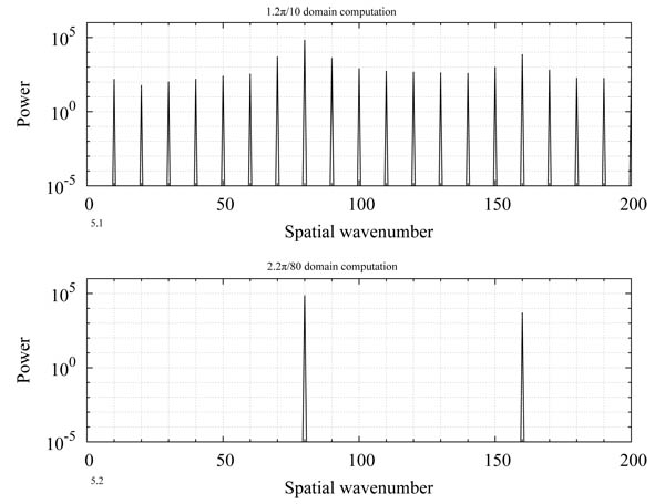 |
Fig. (5). Spatial power spectra of v fluctuations at z = 1.3, T = 6.0 and Re = 600; (1) 2π/10 domain computation, (2) 2π/80 domain computation. |
The vortical structures drawn using the unfiltered data of the 2π/10 computation are shown in Fig. (7.1). The vortical structures obtained by filtering out at particular wavenumber components of 70, 80 and 90 from the same 2π/10 computation are shown in Figs. (7.2, 7.4 and 7.6) respectively. Figs. (7.3, 7.5 and 7.7) show the vortical structures in the narrower computational domain cases (2π/70, 2π/80 and 2π/90), where the data are not filtered. Vortices are visualized using the iso-surface of the second invariant of the velocity gradient tensor Q = 1.0 at T = 6.0. In the wider (2π/10) and narrower (2π/70, 2π/80 and 2π/90) computational domain cases, the numbers of spiral vortices are 80, 70, 80 and 90, respectively. In all cases, the spiral vortices appear from Re = 550 and secondary spiral vortices start to appear around Re = 620 except for the narrower domain case (2π/70), and there are no noticeable differences among the cases. By filtering out at wavenumbers of 70, 80 and 90, it can be found that the spiral vortices corresponding to the wavenumber components of 70, 80 and 90 coexist in the wider domain case (2π/10). The spiral vortices of wavenumber components of 70 and 90 are both much weaker compared to the dominant wavenumber component of 80, and also compared to the wavenumber components of 70 and 90 in the narrower domain cases (2π/70 and 2π/90).
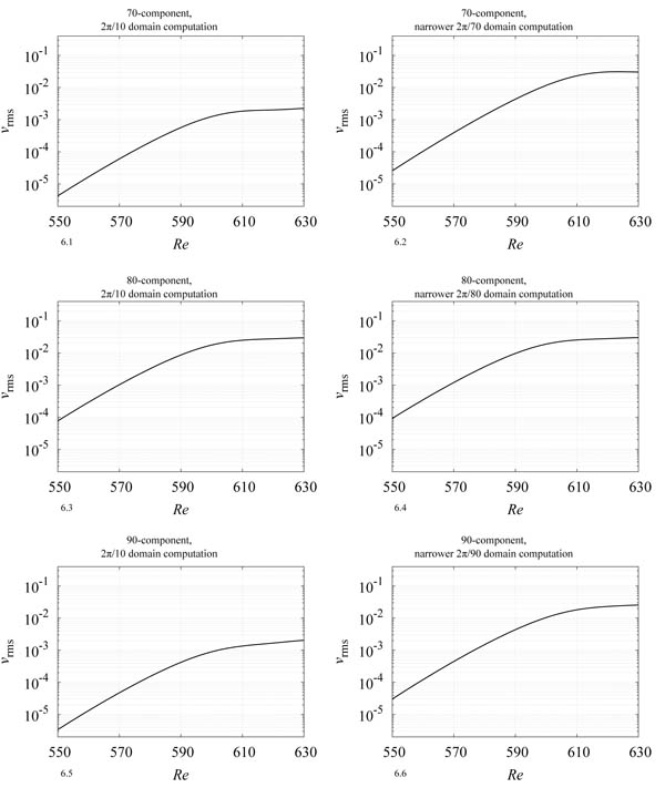 |
Fig. (6). Root mean square of velocity fluctuation measured at the z = 1.3 plane. Each component for the wider domain case (2π/10) and narrower domain cases (2π/70, 2π/80 and 2π/90) is compared. |
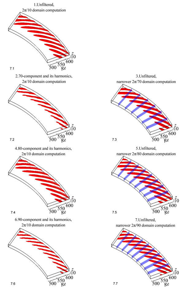 |
Fig. (7). Isosurfaces of Q = 1.0 at T = 6.0; The wider domain case (2π/10) and narrower domain cases (2π/70, 2π/80 and 2π/90) are compared. Blue planes in (3), (5) and (7) denote the borders of the computational domain. |
Next, patterns of spiral vortices corresponding to different azimuthal wavenumbers are compared from a geometric point of view. Fig. (8) provides the definition of an inclination angle of a spiral vortex in the tangential direction, ε. The angle is defined as,
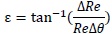 |
(9) |
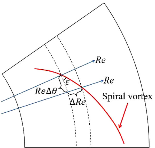 |
Fig. (8). Definition of the angle of spiral vortex ε. The curved line indicates a spiral vortex. ∆Re is the reference unit distance of 1, and ∆θ is the angle between two reference radial axes. |
where ∆θ is the angle between two radial axes, and ∆Re is the reference unit distance, 1.0. Variations in the local angle of spiral vortices are presented in Fig. (9). The angles ε of the spiral vortex decrease monotonically with the Reynolds number. In addition, the vortex angles are smaller for the vortices of smaller wavenumbers. Finally, it is found that the inclined angle in the wider domain computation (2π/10) is close to that of the narrower domain computation in each of the 70, 80 and 90 wavenumber cases.
 |
Fig. (9). Variation in the local angle of a spiral vortex ε by the Reynolds number is shown. Wavenumber components of 70, 80 and 90 of the wider domain case 2π/10 and unfiltered narrower domain cases (2π/70, 2π/80 and 2π/90) are presented. |
Fig. (10) shows the temporal power spectra of the azimuthal velocities at z = 1.3 and Re = 600. The results of the wider (2π/10) and narrower (2π/70, 2π/80 and 2π/90) computational domain cases are compared. The spectra are calculated from 750 data points, which covers T = 3.0 6.0. The data are identical to what a hot wire would measure in an experiment. The horizontal axis in the figure represents the temporal wavenumber, which is the wavenumber per one rotation of the disk. Its resolution is 1/3. Hereafter, we simply call this temporal wavenumber the frequency. As shown in Figs. (10.1, 10.3 and 10.5), the wavenumber components of 70, 80 and 90 in the wider domain computation (2π/10) have non-zero frequencies of 52.33, 59.33 and 65.00, respectively. When the same wavenumber components are compared, there are little differences between frequencies measured in the wider domain case (2π/10) and the narrower domain cases (2π/70, 2π/80 or 2π/90). The frequencies in the rotating frame can be obtained by subtracting each rotational wavenumber from these frequencies in the laboratory frame:
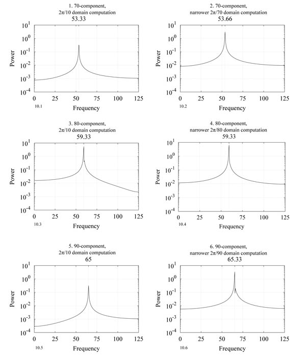 |
Fig. (10). Frequency spectra of v at z = 1.3 and Re = 600, for T = 3.0 ~ 6.0. Wavenumber components of (1) 70, (3) 80 and (5) 90 are filtered out in the wider domain case (2π/10), while wavenumber components of (2) 70, (4) 80, and (6) 90 are filtered out in the narrower domain cases (2π/70, 2π/80, 2π/90), respectively. |
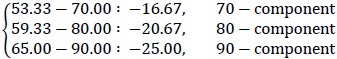 |
The fact that all the values are negative indicates that these wavy patterns are moving in the negative θ direction relative to the rotation of the disk surface. In the case of the wavenumbers 70, 80 or 90, the angle of the spiral vortex and the frequency in the rotating frame are nearly the same between the wider domain computation and the narrower domain computations. This result implies that each of the 70, 80 and 90 wavenumber components in the wider domain (2π/10) computation grew simultaneously due to the global instability. The effect of interactions among the different wavenumber components appears only in the amplitude at which each component saturates. It can be anticipated that the 70 and 90 components in the wider domain case (2π/10) could have grown up to the levels of the higher amplitudes found in the narrower domain computations (2π/70 and 2π/90), if the dominant wavenumber 80 component had not suppressed them through the nonlinear effect.
CONCLUSION
The characteristics of the global instability were investigated using direct numerical simulations. A short-duration wall-normal random suction and blowing was introduced into the Re ≈ 500 ~ 550 area, which was in the stable region for the global instability. Four computations changing the azimuthal size of the domain, 2π/70, 2π/80, 2π/90 and 2π/10, were conducted. In the narrower domain (2π/70, 2π/80, 2π/90) computations, azimuthal wavenumbers that are multiples of the 70, 80 or 90 components, respectively, are likely to appear, whereas in the wider domain (2π/10) case, the azimuthal wavenumber 10 component is likely to appear with its harmonics, such as 10, 20, . . ., 70, 80, 90.
When the artificial disturbance was introduced, it was first convected in the radial direction, but started to grow in response to the global instability, irrespective of the size of the computational domain. Later, at the rotational time of T = 6.0, spiral vortices with an azimuthal wavenumber of 80 became dominant in the flow field in both the wider (2π/10) and narrower (2π/80) computational domain cases. In the wider domain (2π/10) computation, although we expected the appearance of the wavenumber 70 component, which was close to the critical wavenumber of 68 theoretically predicted by Lingwood [13], it was the wavenumber 80 component which actually emerged.
The wavenumber components in each computation were examined. In the narrower domain computations for the 2π/70, 2π/80 and 2π/90 cases, the wavenumber components of 70, 80 and 90 were dominant, respectively. Their strengths were not substantially different. In the wider domain case of 2π/10, the wavenumber 80 component was found to be much stronger than the 70 or 90 components. Comparing the wavenumber 80 components, their strengths in the wider domain computation of 2π/10 and in the narrower domain case of 2π/80 were not very different. So, for each of the wavenumber 70 or 90 components, the strength in the wider domain computation was much lower than that in the narrower domain computation. This result indicated that, in the wider domain computation, the dominant wavenumber 80 component suppressed the wavenumber components of 70 and 90 through a nonlinear effect.
By checking the geometric configuration of the spiral vortices, it was found that, in the wider domain case, vortical structures corresponding to the wavenumber components of 70, 80 and 90 coexisted in the flow field. Comparing the same wavenumber components, there were no differences in the angles of the spiral vortices between the wider and the narrower domain computations.
The frequencies reflecting the rotational speed of the vortical structures were measured, which revealed that all the wavenumber components were moving relative to the disk surface at different speeds depending on the wavenumber. The relative speeds were the same between the wider domain computation and the narrower domain computation.
The results indicated that, in the wider domain computation, although each of the wavenumber 70, 80 and 90 components grew simultaneously due to the global instability, the nonlinear effect caused the wavenumber 80 component to reach a larger amplitude compared to the other two components.
LIST OF ABBREVIATIONS
| u | = perturbation velocities |
| U | = base-flow velocities |
| T | = time |
| p | = pressure |
| f | = forcing term for the sponge regions |
| ν | = kinematic viscosity |
| Ω | = angular velocity |
| ρ | = density |
| T | = the number of disk rotations |
| Re | = Reynolds number |
| ε | = angle of a spiral vortex |
CONSENT FOR PUBLICATION
Not applicable.
CONFLICT OF INTEREST
The authors declare no conflict of interest, financial or otherwise.
ACKNOWLEDGEMENTS
Declared none.